Statistical Mechanics | lecture 1: Introduction and Probability remarks

Full Transcript

https://www.youtube.com/watch?v=5wsja4COMv8

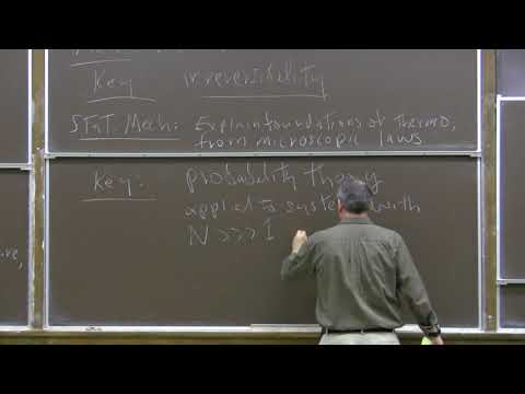
[00:02] Statistical mechanics. I'm John Fresco.
[00:18] Horse has a website different than last.
[00:23] Horse has a website different than last term. It's www.god.caltech.edu/~term.
[00:33] It's www.god.caltech.edu/~term press kill my last name pH 12 see the.
[00:41] Press kill my last name pH 12 see the administrative details are similar to.
[00:43] Administrative details are similar to last term and they're all on the website.
[00:46] That's where the homework will be posted.
[00:49] We have a textbook. It's thermal physics.
[01:02] second edition like at Ellen Cromer I think it's a good book I'll be following it fairly closely we intend to cover chapters 1 through 10 parts of chapter 14 and some extra material that goes beyond the book I'm going to have my sloppy handwritten lecture notes there already they're actually posted on the web and I guess maybe there's going to be video available so you got the notes maybe you have the video so why come to class I mean I'd like you to think of it as the difference this least as far as the notes go between reading Shakespeare and seeing a live performance you know and if you don't think the performance is up to snuff then of course you know.
[02:04] is up to snuff then of course you know what your options are but I really think
[02:08] what your options are but I really think coming to class helps you learn the
[02:10] coming to class helps you learn the stuff but of course that's up to you to
[02:12] stuff but of course that's up to you to decide this is Caltech
[02:13] decide this is Caltech they're all now thermal physics has two
[02:21] they're all now thermal physics has two main components thermodynamics and
[02:30] main components thermodynamics and statistical mechanics
[02:42] what's thermodynamics what we can kind
[02:45] what's thermodynamics what we can kind of characterize it by the main concepts
[02:48] of characterize it by the main concepts it deals with concepts you're familiar
[02:53] it deals with concepts you're familiar with mostly like energy and work and
[03:00] with mostly like energy and work and heat and temperature and most centrally
[03:08] heat and temperature and most centrally of all entropy it has a very clean
[03:18] of all entropy it has a very clean formulation we can kind of boil down the
[03:20] formulation we can kind of boil down the essence of thermodynamics to some
[03:22] essence of thermodynamics to some fundamental principles which can be
[03:24] fundamental principles which can be stated as three or four fundamental laws
[03:36] and that gives the subject two kind of
[03:40] and that gives the subject two kind of pristine beauty there are many
[03:44] pristine beauty there are many applications that won't be our main
[03:48] applications that won't be our main focus in the class which is really to
[03:51] focus in the class which is really to emphasize the foundations but if you
[03:54] emphasize the foundations but if you need motivation for studying the subject
[03:56] need motivation for studying the subject there are a huge number of applications
[03:59] there are a huge number of applications to science technology and actually even
[04:04] to science technology and actually even beyond I'll just say many for now the
[04:12] beyond I'll just say many for now the math is pretty simple the math for
[04:15] math is pretty simple the math for thermodynamics is mostly differential
[04:19] thermodynamics is mostly differential calculus and in particular the calculus
[04:21] calculus and in particular the calculus of functions of several variables so
[04:24] of functions of several variables so many of the mathematical
[04:27] many of the mathematical manipulations involve partial
[04:29] manipulations involve partial derivatives and total derivatives of
[04:35] derivatives and total derivatives of functions of several variables and the
[04:42] functions of several variables and the key to the subject really what we want
[04:47] key to the subject really what we want to gain a deep appreciation of in the
[04:49] to gain a deep appreciation of in the course is the concept of irreversibility
[04:59] the idea that sometimes systems evolve
[05:04] the idea that sometimes systems evolve forward in time in a certain way so that
[05:06] forward in time in a certain way so that if you see a movie of the system
[05:08] if you see a movie of the system evolving backward in time it makes you
[05:10] evolving backward in time it makes you laugh because it's so silly that's their
[05:12] laugh because it's so silly that's their reversibility a guy can jump off the
[05:14] reversibility a guy can jump off the diving board into a swimming pool and
[05:17] diving board into a swimming pool and the energy potential energy release in
[05:19] the energy potential energy release in this fall gets dissipated into the
[05:22] this fall gets dissipated into the molecular motion of the water and so
[05:25] molecular motion of the water and so that's not so funny but when you're on
[05:26] that's not so funny but when you're on it backwards all the molecules push the
[05:29] guy up into the air and onto the diving board and everybody laughs that's
[05:34] board and everybody laughs that's irreversibility and really come while
[05:39] irreversibility and really come while coming back briefly to the applications
[05:41] coming back briefly to the applications the foundations of the subject are
[05:43] the foundations of the subject are really in technology and the importance
[05:47] really in technology and the importance of irreversibility as a limitation on
[05:50] of irreversibility as a limitation on technology the subject was born in the
[05:53] technology the subject was born in the 19th century in efforts to understand
[05:56] 19th century in efforts to understand things like heat engines and the
[05:58] things like heat engines and the applications are things like
[06:01] applications are things like refrigeration as well as many more
[06:03] refrigeration as well as many more esoteric scientific applications
[06:06] esoteric scientific applications understanding phases of matter and so on
[06:08] understanding phases of matter and so on which we'll discuss in detail
[06:14] the other main topic stat mech short for
[06:19] the other main topic stat mech short for statistical mechanics and you can look
[06:24] statistical mechanics and you can look at statistical mechanics as an attempt
[06:26] at statistical mechanics as an attempt to find the deeper principles a
[06:28] to find the deeper principles a successful attempt to find the deeper
[06:31] successful attempt to find the deeper principles underlying thermodynamics
[06:33] principles underlying thermodynamics which explain thermodynamics the central
[06:36] which explain thermodynamics the central achievement of statistical mechanics is
[06:38] achievement of statistical mechanics is to explain thermodynamics on the basis
[06:41] to explain thermodynamics on the basis of microscopic laws governing the
[06:44] of microscopic laws governing the microscopic structure of matter so
[06:47] microscopic structure of matter so explain foundations on thermodynamics
[06:57] from microscopic laws and what's the key
[07:11] from microscopic laws and what's the key to the subject the key is probability
[07:18] to the subject the key is probability theory
[07:25] apply two systems with many degrees of freedom like systems of many particles a gas with an Avogadro's number of molecules in a box applied the systems in which something is large to be concrete I'll say with a very large number of particles like 10 to the 23 or so of the order of Avogadro's number the idea is that we can use probability theory we can compute average properties of systems averaged over many microscopic states and the deviations from that average behavior are rare and small or at least large deviations are rare typical deviations are very small so the average behavior is a very good predictor of how the system will behave and that's what we can compute so what
[08:29] and that's what we can compute so what we do is we predict average behavior and
[08:37] we do is we predict average behavior and observe or mathematically show that big
[08:46] observe or mathematically show that big fluctuations that is big deviations from
[08:49] fluctuations that is big deviations from average behavior are rare and
[08:57] average behavior are rare and persistence with many many particles
[08:58] persistence with many many particles actually very rare so they essentially
[09:01] actually very rare so they essentially never happen and the average behavior
[09:03] never happen and the average behavior really tells us what's going on that's
[09:06] really tells us what's going on that's the idea now notice that here
[09:09] the idea now notice that here probability enters in a rather different
[09:11] probability enters in a rather different way than in the study of quantum
[09:13] way than in the study of quantum mechanics what you learned in physics
[09:16] mechanics what you learned in physics 12b in quantum systems probability is
[09:19] 12b in quantum systems probability is intrinsic even when you have the most
[09:21] intrinsic even when you have the most complete possible description of a
[09:23] complete possible description of a system you're unable to predict except
[09:25] system you're unable to predict except by assigning probabilities the outcome
[09:28] by assigning probabilities the outcome of measurement okay you couldn't
[09:31] of measurement okay you couldn't possibly know more about the system you
[09:33] possibly know more about the system you still can't predict what will happen
[09:34] still can't predict what will happen when you measure it that's not what
[09:36] when you measure it that's not what we're talking about here what we're
[09:38] we're talking about here what we're talking about
[09:39] talking about is that probability arises in practice
[09:42] is that probability arises in practice because we don't have a complete
[09:44] because we don't have a complete description of the system there are many
[09:46] description of the system there are many possible microscopic states we don't
[09:47] possible microscopic states we don't know which one but we don't need to know
[09:49] know which one but we don't need to know which one because all these microscopic
[09:51] which one because all these microscopic states that occur with reasonable
[09:53] states that occur with reasonable likelihood lead to similar behavior
[09:59] [Music]
[10:02] [Music] so I'll just say unlike quantum
[10:07] so I'll just say unlike quantum mechanics as in physics 12b this is
[10:16] mechanics as in physics 12b this is probability arises in practice because
[10:27] probability arises in practice because we don't have complete knowledge of the
[10:35] we don't have complete knowledge of the system's actual state not in principle.
[10:43] system's actual state not in principle as in the quantum measurement process.
[10:51] what's the math well it's probability.
[10:57] what's the math well it's probability theory.
[11:03] and really it's counting counting the.
[11:13] and really it's counting counting the number of states that a system can be in.
[11:15] number of states that a system can be in subject to constraints sounds simple but it's not always simple sometimes.
[11:18] it's not always simple sometimes counting is hard conceptually it's simple in practice it can be hard now.
[11:26] these two pillars of thermal physics statistical mechanics and thermodynamics.
[11:30] statistical mechanics and thermodynamics which are of course closely related as I've already emphasized in physics 12c.
[11:36] I've already emphasized in physics 12c our emphasis will be on statistical.
[11:37] Our emphasis will be on statistical mechanics well talk about thermodynamics.
[11:41] Mechanics well talk about thermodynamics we'll see how it emerges from the.
[11:43] We'll see how it emerges from the statistical mechanical picture of the.
[11:46] Statistical mechanical picture of the world but our main goal will be to.
[11:48] World but our main goal will be to understand the foundations and.
[11:50] Understand the foundations and applications of statistical mechanics.
[11:53] And it's really a great subject for.
[11:56] And it's really a great subject for physics 12 because from a few fairly.
[12:00] Physics 12 because from a few fairly clear conceptually and accessible.
[12:03] Clear conceptually and accessible principles and methods we can understand.
[12:06] Principles and methods we can understand a lot of physics and that's what we'll.
[12:08] A lot of physics and that's what we'll try to do in this course now statistical.
[12:12] Try to do in this course now statistical mechanics the focus of.
[12:28] The 612 C is also an extremely active.
[12:32] The 612 C is also an extremely active subject of contemporary physics much of.
[12:36] subject of contemporary physics much of what physicists call the study of
[12:38] what physicists call the study of condensed matter which means solid state
[12:45] condensed matter which means solid state systems and systems of well systems of
[12:49] systems and systems of well systems of many particles in various settings much
[12:56] many particles in various settings much of those studies are based on
[12:57] of those studies are based on applications of statistical mechanics to
[13:01] applications of statistical mechanics to things like the different kinds of
[13:04] things like the different kinds of phases and phase transitions one of the
[13:06] phases and phase transitions one of the things we'll be talking about
[13:08] things we'll be talking about transitions between phases to different
[13:11] transitions between phases to different classes of materials and various ways of
[13:16] classes of materials and various ways of classifying the properties of systems
[13:18] classifying the properties of systems with many particles okay so let's start
[13:31] with many particles okay so let's start counting any questions about all this so
[13:35] counting any questions about all this so far
[13:43] so let's start to familiarize ourselves
[13:46] so let's start to familiarize ourselves with the main idea that we're going to
[13:49] with the main idea that we're going to use throughout the course it's a simple
[13:51] idea we have some system maybe it's a gas
[14:06] the important thing is it has many degrees of freedom let's say many
[14:10] degrees of freedom let's say many molecules in a box it's my picture of gas in a box
[14:12] molecules in a box it's my picture of gas in a box
[14:16] we specify some macroscopic property of the system that we can imagine measuring or characterizing the system
[14:20] property of the system that we can imagine measuring or characterizing the system
[14:22] like for example the total energy
[14:26] system like for example the total energy
[14:28] now specify a macroscopic property like the total energy we don't specify it
[14:41] now specify a macroscopic property like the total energy we don't specify it
[14:48] the total energy we don't specify it exactly to an infinite number of digits
[14:51] exactly to an infinite number of digits of precision but to some approximation
[14:53] of precision but to some approximation so we say e is a lower bound on the
[15:00] so we say e is a lower bound on the total energy say and II plus Delta e has
[15:10] total energy say and II plus Delta e has not profound the energy is in between
[15:11] not profound the energy is in between it's in that range somewhere okay that's
[15:13] it's in that range somewhere okay that's what I mean by specifying a macroscopic
[15:15] what I mean by specifying a macroscopic quantity and of all the states that have
[15:18] quantity and of all the states that have energy in this range well there are many
[15:20] energy in this range well there are many of them lots and lots of microscopic
[15:22] of them lots and lots of microscopic states lots of ways in which that energy
[15:24] states lots of ways in which that energy could be shared as kinetic energy among
[15:27] could be shared as kinetic energy among the different molecules in the box and
[15:30] the different molecules in the box and now we're trying to understand what's
[15:33] now we're trying to understand what's going on in the box we're going to rely
[15:36] going on in the box we're going to rely on an assumption which I'm not really
[15:38] on an assumption which I'm not really going to justify from first principles
[15:40] going to justify from first principles because doing so is actually not easy so
[15:45] because doing so is actually not easy so let's be honest and state it as an
[15:46] let's be honest and state it as an assumption
[15:51] which is all microscopic states which
[16:03] which is all microscopic states which are consistent with I'll call it our
[16:09] are consistent with I'll call it our macroscopic specification I don't know
[16:12] macroscopic specification I don't know it's kind of an awkward way of saying it
[16:14] it's kind of an awkward way of saying it and I've already said it in this case
[16:18] and I've already said it in this case our statement that the total energy is
[16:21] our statement that the total energy is in a certain range all microscopic
[16:24] in a certain range all microscopic states are equally likely
[16:32] it's very egalitarian democratic
[16:35] it's very egalitarian democratic principle all the microscopic states
[16:37] principle all the microscopic states have an equal right to be the
[16:39] have an equal right to be the microscopic state of the system as long
[16:42] microscopic state of the system as long as they're consistent with whatever it
[16:43] as they're consistent with whatever it is we know or we specify like for
[16:45] is we know or we specify like for example the total energy so that means
[16:49] example the total energy so that means each one of those states we don't we're
[16:52] each one of those states we don't we're saying we're pleading ignorance we don't.
[16:53] saying we're pleading ignorance we don't know anything about the microscopic state.
[16:54] know anything about the microscopic state so we might as well assume that.
[16:57] state so we might as well assume that there's a uniform probability distribution in all the states.
[16:58] there's a uniform probability distribution in all the states each one of them by a microscopic state I mean.
[17:01] distribution in all the states each one of them by a microscopic state I mean say specifying the position and velocity of all the molecules in the box can't.
[17:05] say specifying the position and velocity of all the molecules in the box can't really do that in quantum mechanics.
[17:10] of all the molecules in the box can't really do that in quantum mechanics we'll come back to that but anyway some way of completely characterizing state.
[17:13] really do that in quantum mechanics we'll come back to that but anyway some way of completely characterizing state.
[17:14] we'll come back to that but anyway some way of completely characterizing state and the probability of a state in other words is given by a uniform distribution.
[17:17] way of completely characterizing state and the probability of a state in other words is given by a uniform distribution.
[17:19] and the probability of a state in other words is given by a uniform distribution for every state it's just 1 over the total number of states.
[17:23] words is given by a uniform distribution for every state it's just 1 over the total number of states.
[17:26] for every state it's just 1 over the total number of states and actually quantum mechanics helps us here.
[17:28] and actually quantum mechanics helps us here it helps us by allowing us to count states.
[17:43] and actually quantum mechanics helps us here.
[17:46] here it helps us by allowing us to count states.
[17:46] it helps us by allowing us to count states states are discrete in quantum mechanics at least if we have a system.
[17:48] states states are discrete in quantum mechanics at least if we have a system.
[17:51] states states are discrete in quantum mechanics at least if we have a system.
[17:54] mechanics at least if we have a system which has a finite volume a finite size
[17:58] which has a finite volume a finite size then there's some Hamiltonian say which
[18:03] then there's some Hamiltonian say which characterizes the state and it has a
[18:06] characterizes the state and it has a spectrum of eigen values right you
[18:08] spectrum of eigen values right you learned all about that in 12b all the
[18:11] learned all about that in 12b all the stationary states they're actually a
[18:13] stationary states they're actually a finite number of them in an energy range
[18:15] finite number of them in an energy range Princeton principle you can count them
[18:17] Princeton principle you can count them all and classical mechanics it's a
[18:19] all and classical mechanics it's a little harder to say although you can do
[18:21] little harder to say although you can do it exactly what you mean by counting
[18:23] it exactly what you mean by counting States is there really a continuum of
[18:24] States is there really a continuum of states in quantum mechanics states are
[18:28] states in quantum mechanics states are really discrete which makes it easier to
[18:30] really discrete which makes it easier to give a rigorous version of what we mean
[18:33] give a rigorous version of what we mean by counting States and quantum mechanics
[18:38] by counting States and quantum mechanics states really are discrete and so can be
[18:49] states really are discrete and so can be counted at least if we don't have an
[18:54] counted at least if we don't have an infinite system in practice we never do
[18:59] Infinite system in practice we never do and so I've already told you what we're.
[19:03] And so I've already told you what we're going to do we're going to compute average behavior.
[19:04] So our job as I've already said but it's worth saying again it's twofold.
[19:14] It's twofold compute average behavior for this ensemble of possible microscopic states and verify that large fluctuations away from the average behavior are very rare.
[20:15] so the typical behavior the system
[20:17] so the typical behavior the system really is like we would predict by
[20:20] really is like we would predict by considering average behavior averaged
[20:22] considering average behavior averaged over this uniform ensemble well you
[20:40] over this uniform ensemble well you probably know what I mean by the
[20:43] probably know what I mean by the fluctuations being small we don't with
[20:46] fluctuations being small we don't with large fluctuations being rare but let's
[20:49] large fluctuations being rare but let's discuss that to remind ourselves what it
[20:54] discuss that to remind ourselves what it means let's start with about the
[20:59] means let's start with about the simplest example we can think of which
[21:01] simplest example we can think of which is we have a fair coin okay flip it it
[21:05] is we have a fair coin okay flip it it comes up heads with probability 1/2 and
[21:07] comes up heads with probability 1/2 and tails with probability 1/2
[21:09] tails with probability 1/2
[21:22] so if we plot probability as a function
[21:29] so if we plot probability as a function of the number of heads that come up the
[21:34] of the number of heads that come up the number of heads can be either 0 over 1
[21:36] number of heads can be either 0 over 1 it's a flat distribution both heads and
[21:40] it's a flat distribution both heads and tails have probability 1/2 probability
[21:43] tails have probability 1/2 probability 1/2 for zero heads if I flip it once
[21:46] 1/2 for zero heads if I flip it once probability 1/2 for 1 heads that's for
[21:50] probability 1/2 for 1 heads that's for one coin but I'm interested in what
[21:52] one coin but I'm interested in what happens when I flip a lot of coins well
[21:57] happens when I flip a lot of coins well let's start with two just so we
[21:58] let's start with two just so we understand what we're doing if I have
[22:00] understand what we're doing if I have two coins each one comes up heads or
[22:06] two coins each one comes up heads or tails there are eight sorry for I jumped
[22:08] tails there are eight sorry for I jumped ahead to three coins there are four
[22:10] ahead to three coins there are four possibilities for what can happen we can
[22:13] possibilities for what can happen we can get tails twice tails and then heads
[22:16] get tails twice tails and then heads heads and then tails or heads twice so
[22:20] heads and then tails or heads twice so here we get no heads these are the two
[22:22] here we get no heads these are the two ways of getting one heads and there's
[22:25] ways of getting one heads and there's one way of getting two heads so if I
[22:29] one way of getting two heads so if I divide by four so I get a normalized
[22:31] divide by four so I get a normalized probability the probability as a
[22:34] probability the probability as a function of the number of heads looks
[22:41] function of the number of heads looks like this
[22:44] oh sorry I'm Tim jumped ahead again
[22:51] stuff so purchase two coins we're gonna
[22:58] stuff so purchase two coins we're gonna have either 0 1 or 2 with probability
[23:02] have either 0 1 or 2 with probability 1/4 of having 0 or 2 and probability 1/2
[23:06] 1/4 of having 0 or 2 and probability 1/2 of getting two heads and we can keep
[23:09] of getting two heads and we can keep going
[23:10] going right if I consider three coins there
[23:21] right if I consider three coins there are eight possible outcomes when I flip
[23:22] are eight possible outcomes when I flip a coin three times if it's a fair coin
[23:25] a coin three times if it's a fair coin then they're actually three ways of
[23:30] then they're actually three ways of getting a one heads three ways of
[23:33] getting a one heads three ways of getting two heads one way of getting
[23:37] getting two heads one way of getting three heads one way of getting zero
[23:39] three heads one way of getting zero heads the probability distribution looks
[23:41] heads the probability distribution looks like this where these probabilities are
[23:47] like this where these probabilities are 1/8 then these are 3/8 all right so now
[23:54] 1/8 then these are 3/8 all right so now I'm going to imagine I flip n coins and
[23:57] I'm going to imagine I flip n coins and n is a large number 1 2 3 many
[24:03] n is a large number 1 2 3 many [Music]
[24:25] well now there are lots of possible
[24:27] well now there are lots of possible outcomes flip the coin n times they're 2
[24:31] outcomes flip the coin n times they're 2 to the N possibilities well you know
[24:49] that on average the number of times I'm
[24:53] that on average the number of times I'm going to get a heads is 1/2 of the time
[24:58] going to get a heads is 1/2 of the time now the most likely possibility for the
[25:01] now the most likely possibility for the number of heads is actually n over 2 and
[25:03] number of heads is actually n over 2 and I round down over 2 there's a
[25:05] I round down over 2 there's a distribution and it looks kind of like
[25:07] distribution and it looks kind of like that and in fact in a sense which will
[25:14] that and in fact in a sense which will make precise this distribution becomes
[25:17] make precise this distribution becomes very narrow as n gets large it has a
[25:29] very narrow as n gets large it has a characteristic shape which we call a
[25:34] characteristic shape which we call a Gaussian or a normal distribution and
[25:44] Gaussian or a normal distribution and actually this is a special case of a
[25:46] actually this is a special case of a rather general result called the central
[25:49] rather general result called the central limit theorem
[26:05] the central limit theorem actually says
[26:07] the central limit theorem actually says this consider any probability
[26:11] this consider any probability distribution this has some nice
[26:14] distribution this has some nice mathematical properties but let's assume
[26:16] mathematical properties but let's assume that it does so let t be some variable
[26:23] that it does so let t be some variable it was 0 & 1 in the case where I flipped
[26:26] it was 0 & 1 in the case where I flipped a single coin and I assign a probability
[26:30] a single coin and I assign a probability to each value of T and so there's some
[26:33] to each value of T and so there's some distribution here it is okay
[26:37] distribution here it is okay that's some crazy shape maybe but now we
[26:40] that's some crazy shape maybe but now we sample from this distribution many times
[26:42] sample from this distribution many times so that means weighted by the
[26:44] so that means weighted by the probability I choose some particular
[26:46] probability I choose some particular value of T each time I take a sample and
[26:49] value of T each time I take a sample and I do that end times and then let's
[27:00] I do that end times and then let's consider the sum over those and samples
[27:05] consider the sum over those and samples of the value of T in each sample I'll
[27:08] of the value of T in each sample I'll call that capital T sub n because I
[27:12] call that capital T sub n because I sampled n times the sum of the result
[27:16] sampled n times the sum of the result when I sample the first time plus the
[27:18] when I sample the first time plus the second time up to the nth time and then
[27:24] second time up to the nth time and then I ask what's the distribution for the
[27:27] I ask what's the distribution for the sum so in fact when n gets large the
[27:34] sum so in fact when n gets large the probability distribution
[27:41] or T sub n approaches a Gaussian a
[27:47] or T sub n approaches a Gaussian a narrow Gaussian like going for the coins
[27:56] when n is large that's what I mean by
[28:02] when n is large that's what I mean by the central limit theorem I'm not going
[28:04] the central limit theorem I'm not going to give a proof of the central limit
[28:06] to give a proof of the central limit theorem but let's look at how it applies
[28:09] theorem but let's look at how it applies in more detail to the case of flipping a
[28:11] in more detail to the case of flipping a fair coin and times
[28:20] [Music]
[28:54] except I just remembered something this
[28:57] except I just remembered something this is a physics class okay so I'm going to
[29:00] is a physics class okay so I'm going to make it sound like physics by saying
[29:03] make it sound like physics by saying instead of flipping coins I have a model
[29:06] instead of flipping coins I have a model of a magnet now there's a big hunk of
[29:20] of a magnet now there's a big hunk of magnetic material and in that material
[29:24] magnetic material and in that material there are a lot of spins maybe their
[29:26] there are a lot of spins maybe their electron spins I guess you know
[29:30] electron spins I guess you know electrons have spin and let's say each
[29:35] electrons have spin and let's say each one of those spins can point either up
[29:38] one of those spins can point either up or down along the vertical axis okay
[29:46] there's a spin at each of and sites in
[29:55] there's a spin at each of and sites in our magnetic material each is either
[30:03] our magnetic material each is either spin up or spin down and let's suppose
[30:09] spin up or spin down and let's suppose that there's no particular reason for us
[30:12] that there's no particular reason for us then to prefer to point up or down so it
[30:15] then to prefer to point up or down so it decides at random whether to point up or
[30:22] decides at random whether to point up or down for each spin independently
[30:28] it has probability 1/2 of pointing up
[30:30] it has probability 1/2 of pointing up and probability 1/2 for pointing down
[30:33] and probability 1/2 for pointing down well it's a lot like the coins right
[30:35] well it's a lot like the coins right there like coins which I flipped with
[30:37] there like coins which I flipped with her which are either heads or tails now
[30:40] her which are either heads or tails now each one of those spins actually has a
[30:42] each one of those spins actually has a magnetic moment and what we call the
[30:44] magnetic moment and what we call the magnetization in our magnet is the sum
[30:47] magnetization in our magnet is the sum with a sign the difference between the
[30:50] with a sign the difference between the magnetization due to all the spins which
[30:52] magnetization due to all the spins which are up and the magnetization due to all
[30:55] are up and the magnetization due to all the spins that are down the
[30:57] the spins that are down the magnetization I'll call it capital M is
[31:07] magnetization I'll call it capital M is the number of up spins minus the number
[31:10] the number of up spins minus the number of down spins times the magnetic moment
[31:13] of down spins times the magnetic moment of a single spin
[31:24] the magnetization is just the magnetic
[31:28] the magnetization is just the magnetic moment of the whole sample if half the
[31:30] moment of the whole sample if half the spins were up and half the spins were
[31:32] spins were up and half the spins were down their magnetic moments which cancel
[31:34] down their magnetic moments which cancel out but there might just by chance be in
[31:36] out but there might just by chance be in excess of either up over down or down
[31:38] excess of either up over down or down over up and as a result there will be
[31:40] over up and as a result there will be some non-zero magnetization for my bulk
[31:44] some non-zero magnetization for my bulk magnetic material some big hunk of
[31:46] magnetic material some big hunk of magnet with Avogadro's number of spins
[31:48] magnet with Avogadro's number of spins in it so suppose the magnetization in
[31:53] in it so suppose the magnetization in this case is the macroscopic quantity
[31:56] this case is the macroscopic quantity that we're going to fix if somebody can
[31:57] that we're going to fix if somebody can come along and measure it okay with a
[31:59] come along and measure it okay with a magnetometer that's the macroscopic
[32:11] magnetometer that's the macroscopic quantity which we specify and we like to
[32:21] quantity which we specify and we like to kind of understand from first principles
[32:23] kind of understand from first principles what to expect when we measure the
[32:25] what to expect when we measure the magnetization okay at least what's
[32:28] magnetization okay at least what's predicted by this model
[32:34] so actually I can write the
[32:36] so actually I can write the magnetization it's convenient to write
[32:40] magnetization it's convenient to write it as something I'll call to us times
[32:44] it as something I'll call to us times the magnetic moment this is just to give
[32:47] the magnetic moment this is just to give it a name I'll call it the spin excess
[32:50] it a name I'll call it the spin excess so in other words I can write the number
[32:52] so in other words I can write the number of up spins as half of the spins plus s
[32:58] of up spins as half of the spins plus s and the number of down spins is half of
[33:02] and the number of down spins is half of the spins minus s the sum is n and the
[33:08] the spins minus s the sum is n and the difference between the number up and the
[33:09] difference between the number up and the number down is to us let me call a
[33:17] number down is to us let me call a number G the multiplicity of that
[33:24] number G the multiplicity of that particular value of the magnetization it
[33:26] particular value of the magnetization it means the number of possible states of
[33:29] means the number of possible states of our magnet we're in a state i specify
[33:31] our magnet we're in a state i specify for every one of the in spins whether
[33:33] for every one of the in spins whether it's up or down this multiplicity is the
[33:36] it's up or down this multiplicity is the number of states
[33:44] Oh with spin excess to us a specified
[33:53] Oh with spin excess to us a specified value of s and n spends total and I'd
[34:04] value of s and n spends total and I'd like to compute what that is so it's
[34:09] like to compute what that is so it's just the same mathematical question is
[34:11] just the same mathematical question is asking how many ways when I flip the
[34:14] asking how many ways when I flip the coin 10 times are there to get a number
[34:17] coin 10 times are there to get a number of heads which is half of all the flips
[34:19] of heads which is half of all the flips plus s same thing but I made it sound
[34:23] plus s same thing but I made it sound like physics
[34:28] [Music]
[35:07] okay so really we just have to find
[35:11] okay so really we just have to find binomial coefficients we think of each
[35:15] binomial coefficients we think of each time we look at it spin it can be either
[35:17] time we look at it spin it can be either up or down there are n spins so we can
[35:22] up or down there are n spins so we can think of 2 to the N possible sequences
[35:26] think of 2 to the N possible sequences binary sequences if you think of up and
[35:29] binary sequences if you think of up and down as 0 & 1 each sequence specifies
[35:33] down as 0 & 1 each sequence specifies which spins are up which bends are down
[35:34] which spins are up which bends are down I want to count all the sequences which
[35:37] I want to count all the sequences which have a specified spin XS so they're all
[35:42] have a specified spin XS so they're all together 2 to the n states each one is
[35:52] together 2 to the n states each one is either up or down out of N and how many
[35:55] either up or down out of N and how many of them have a specified spin XS and
[36:02] of them have a specified spin XS and what I mean by the multiplicity is the
[36:08] what I mean by the multiplicity is the number of terms the number of sequences
[36:12] number of terms the number of sequences all its sequences with a specified
[36:19] all its sequences with a specified number of up spins as I already said 1/2
[36:24] number of up spins as I already said 1/2 n plus s and the rest down which means
[36:28] n plus s and the rest down which means they're 1/2 and minus s which are down
[36:31] they're 1/2 and minus s which are down and that's just equal to the number of
[36:37] and that's just equal to the number of ways of choosing and up up spins out of
[36:43] ways of choosing and up up spins out of all together n spins right which I can
[36:48] all together n spins right which I can write as n factorial divided by the
[36:51] write as n factorial divided by the number up factorial divided by the
[36:54] number up factorial divided by the number down factorial that's because n
[36:58] number down factorial that's because n factorial is the number of ways I can
[37:02] factorial is the number of ways I can permute all the bits in the sequence but
[37:06] permute all the bits in the sequence but an up factorial of those permutations
[37:09] an up factorial of those permutations just mix up the up spins with one
[37:11] just mix up the up spins with one another and that doesn't change the
[37:13] another and that doesn't change the state doesn't change the configuration
[37:15] state doesn't change the configuration so I divide by that and and down
[37:18] so I divide by that and and down factorial of the permutations the
[37:20] factorial of the permutations the permutations of all the down spins
[37:21] permutations of all the down spins doesn't change the configuration because
[37:23] doesn't change the configuration because it just permutes down spins with one
[37:25] it just permutes down spins with one another right so let's just write out
[37:33] another right so let's just write out what it is and factorial divided by and
[37:40] what it is and factorial divided by and over two plus s factorial and over two
[37:46] over two plus s factorial and over two minus s factorial we want to understand
[37:52] minus s factorial we want to understand how that quantity behaves as s varies
[37:54] how that quantity behaves as s varies and to do that we're going to make an
[37:57] and to do that we're going to make an approximation because we would like to
[38:03] approximation because we would like to see the sharp Gaussian emerging from
[38:05] see the sharp Gaussian emerging from this description I'm going to suppose
[38:11] this description I'm going to suppose that s is small compared to n well
[38:16] that s is small compared to n well actually we'll be able to justify that
[38:17] actually we'll be able to justify that in retrospect when we see what the
[38:19] in retrospect when we see what the answer is it's just saying that the very
[38:21] answer is it's just saying that the very large fluctuations are extremely rare so
[38:23] large fluctuations are extremely rare so forget about them we're only going to
[38:26] forget about them we're only going to have to study the small fluctuations in
[38:27] have to study the small fluctuations in which the spin excess is small compared
[38:30] which the spin excess is small compared to the total number of spins
[38:45] and we'll make another approximation in
[38:49] and we'll make another approximation in evaluating n factorial the Stirling
[38:52] evaluating n factorial the Stirling approximation and factorial can be
[39:04] approximation and factorial can be written as 2 pi n to the 1/2 power n to
[39:12] written as 2 pi n to the 1/2 power n to the power n e to the minus n plus some
[39:21] the power n e to the minus n plus some stuff in the exponential that becomes
[39:23] stuff in the exponential that becomes unimportant when n is large I can expand
[39:32] unimportant when n is large I can expand that exponential but we're going to
[39:34] that exponential but we're going to ignore all these Corrections that means
[39:40] ignore all these Corrections that means we'll have the right answer up to some
[39:42] we'll have the right answer up to some factor which is the exponential of this
[39:44] factor which is the exponential of this number which is very close to 0 up to
[39:47] number which is very close to 0 up to some factor which is very close to 1
[39:49] some factor which is very close to 1 okay and if you haven't seen the
[39:53] okay and if you haven't seen the derivation of the Stirling approximation
[39:55] derivation of the Stirling approximation it's it's in Appendix A of the book it's
[39:59] it's it's in Appendix A of the book it's very easy to understand the end of the
[40:00] very easy to understand the end of the nd to the minus sign you have to work a
[40:02] nd to the minus sign you have to work a little harder to get the 2 pi n to the 1
[40:05] little harder to get the 2 pi n to the 1 hat which actually isn't all that
[40:07] hat which actually isn't all that important anyway but to understand the
[40:12] important anyway but to understand the terms that are important just note
[40:15] terms that are important just note consider taking the log of n factorial
[40:18] consider taking the log of n factorial the log of n factorial let's say the
[40:23] the log of n factorial let's say the natural log of n factorial the natural
[40:27] natural log of n factorial the natural log of the product from M equals 1 to n
[40:30] log of the product from M equals 1 to n because that's what a factorial is of M
[40:33] because that's what a factorial is of M taking the log of the product becomes
[40:35] taking the log of the product becomes the sum of the logs
[40:42] and when n is very large we can
[40:47] and when n is very large we can approximate the sum by an integral
[40:48] approximate the sum by an integral fairly well up to some additive factor
[40:51] fairly well up to some additive factor which is of order one so it's like
[40:53] which is of order one so it's like integrating 1/2 m DN log m and you know
[40:58] integrating 1/2 m DN log m and you know how to do that integral its M log M
[41:02] how to do that integral its M log M minus M valuated it and and 1 the
[41:08] minus M valuated it and and 1 the contribution from the lower limit of
[41:10] contribution from the lower limit of integration isn't too important
[41:12] integration isn't too important so it's essentially n log n minus N and
[41:17] so it's essentially n log n minus N and what I have here in N to the NT to the
[41:19] what I have here in N to the NT to the minus n is the exponential of that and
[41:22] minus n is the exponential of that and like I said with a little more work you
[41:24] like I said with a little more work you can get the 2 pi n to the 1/2
[41:42] [Music]
[41:56] okay so let's just plug in to the
[42:00] okay so let's just plug in to the Sterling approximation the factorials
[42:03] Sterling approximation the factorials that were that we want to evaluate here
[42:06] that were that we want to evaluate here maybe it'll be helpful to write this as
[42:09] maybe it'll be helpful to write this as n factorial divided by let's factor out
[42:14] n factorial divided by let's factor out and then over two times one plus two us
[42:18] and then over two times one plus two us over n factorial and n over 2 1 minus
[42:25] over n factorial and n over 2 1 minus two us over n factorial and apply
[42:32] two us over n factorial and apply Sterling's approximation to that so for
[42:44] Sterling's approximation to that so for the n factorial in the numerator I have
[42:46] the n factorial in the numerator I have two pi n to the one half n to the N e to
[42:52] two pi n to the one half n to the N e to the minus n and then for the first
[43:00] the minus n and then for the first factor in the denominator
[43:02] factor in the denominator because it's in the denominator I turn
[43:05] because it's in the denominator I turn everything upside down so it becomes a 2
[43:09] everything upside down so it becomes a 2 pi times 1/2 n 1 plus 2 s over N to the
[43:15] pi times 1/2 n 1 plus 2 s over N to the minus 1/2 and then n over 2 1 plus 2 s
[43:23] minus 1/2 and then n over 2 1 plus 2 s over N raised to the power because it's
[43:27] over N raised to the power because it's in the denominator minus n over 2 1 plus
[43:31] in the denominator minus n over 2 1 plus 2 s over n and then for the other factor
[43:36] 2 s over n and then for the other factor in the denominator 2 pi 1/2 n 1 minus 2
[43:43] in the denominator 2 pi 1/2 n 1 minus 2 s over n to the minus 1/2
[43:48] s over n to the minus 1/2 and over 2 1 minus 2 s over N raised to
[43:56] and over 2 1 minus 2 s over N raised to the power because it's in the
[43:57] the power because it's in the denominator minus n over 2 times a 1
[44:02] denominator minus n over 2 times a 1 minus 2 s over N except I guess I also
[44:06] minus 2 s over N except I guess I also forgot the exponential but here would be
[44:09] forgot the exponential but here would be e to the N over 2 times 1 plus 2 s over
[44:15] e to the N over 2 times 1 plus 2 s over N and here would be e to the N over 2
[44:18] N and here would be e to the N over 2 because it's in the denominator 1 minus
[44:21] because it's in the denominator 1 minus 2 s over n don't you need to multiply
[44:25] 2 s over n don't you need to multiply together all these factors that's not in
[44:27] together all these factors that's not in the exponent it looked like it was so
[44:31] the exponent it looked like it was so I'll rewrite it e to the N over 2 1
[44:35] I'll rewrite it e to the N over 2 1 minus 2 s over well when I multiply this
[44:40] minus 2 s over well when I multiply this exponential times this 1 this annoying 2
[44:43] exponential times this 1 this annoying 2 s over N goes away and then I have an e
[44:46] s over N goes away and then I have an e to the end but that cancels the e to the
[44:48] to the end but that cancels the e to the minus n so I can get rid of all that
[44:50] minus n so I can get rid of all that junk and then I have an end to the N and
[44:57] junk and then I have an end to the N and here I have an N to the minus n over 2
[45:01] here I have an N to the minus n over 2 times 1 plus 2 s over N and here and n
[45:03] times 1 plus 2 s over N and here and n to the minus n over 2 1 minus 2 s over n
[45:06] to the minus n over 2 1 minus 2 s over n and so that all cancels to okay so I can
[45:10] and so that all cancels to okay so I can get rid of that and that and then and
[45:15] get rid of that and that and then and then I guess I should combine together
[45:18] then I guess I should combine together the two pies and stuff
[45:22] [Music]
[45:27] so I had a 2pi in the numerator but I
[45:31] so I had a 2pi in the numerator but I had two two pies in the denominator
[45:32] had two two pies in the denominator all to the one-half power so it's two pi
[45:53] all to the one-half power so it's two pi to the minus 1/2 and then well there's
[45:58] to the minus 1/2 and then well there's this 1/2 raised to the minus 1/2 and
[46:01] this 1/2 raised to the minus 1/2 and then another 1/2 raised to the minus 1/2
[46:03] then another 1/2 raised to the minus 1/2 it's all together that's a two and an
[46:09] it's all together that's a two and an end to the one-half and two and to the
[46:12] end to the one-half and two and to the minus 1/2 so that gives me and then to
[46:15] minus 1/2 so that gives me and then to the minus 1/2 now I got this 1/2 here
[46:23] the minus 1/2 now I got this 1/2 here and it gets raised to this power so I
[46:26] and it gets raised to this power so I have 1/2 raised to that power times 1/2
[46:29] have 1/2 raised to that power times 1/2 raised to that power and that gets rid
[46:31] raised to that power and that gets rid of those 2's over and Corrections so
[46:33] of those 2's over and Corrections so that just gives me a 2 to the N and then
[46:38] that just gives me a 2 to the N and then let's look at what we have left we've
[46:40] let's look at what we have left we've just got the 1 plus 2's over N to a
[46:43] just got the 1 plus 2's over N to a power the 1 minus 2's over N to a power
[46:45] power the 1 minus 2's over N to a power we also had the product of these two
[46:48] we also had the product of these two factors that's not important actually
[46:51] factors that's not important actually but I do want to keep track of the 1
[46:54] but I do want to keep track of the 1 plus 2's over N to the power minus n
[46:58] plus 2's over N to the power minus n over 2 1 plus 2's over N and then 1
[47:04] over 2 1 plus 2's over N and then 1 minus 2's over N to the power minus n
[47:10] minus 2's over N to the power minus n over 2 1 minus 2's over N and that last
[47:15] over 2 1 minus 2's over N and that last factor which I'm actually not going to
[47:18] factor which I'm actually not going to worry about which is this 1 plus 2's
[47:20] worry about which is this 1 plus 2's over n times this 1 minus 2's over N
[47:23] over n times this 1 minus 2's over N which is all together 1 minus 4s squared
[47:29] which is all together 1 minus 4s squared over N squared to the minus 1/2
[47:34] over N squared to the minus 1/2 but I'm just going to approximate that
[47:35] but I'm just going to approximate that by one because remember we're going to
[47:37] by one because remember we're going to assume that that's small okay so the
[47:42] assume that that's small okay so the only thing we have to work on a little
[47:43] only thing we have to work on a little bit more is this product of factors at
[47:47] bit more is this product of factors at this point it's handy to take the
[47:49] this point it's handy to take the logarithm and then after we get the
[47:55] logarithm and then after we get the result we can exponentiate it so what
[48:04] result we can exponentiate it so what I'm taking the logarithm of is this
[48:09] I'm taking the logarithm of is this times this and so I have minus n over 2
[48:24] times this and so I have minus n over 2 1 plus 2 s over n times the log of 1
[48:29] 1 plus 2 s over n times the log of 1 plus 2 s over end from the first factor
[48:34] plus 2 s over end from the first factor when I take its log and and then I get
[48:36] when I take its log and and then I get the same thing but with s replaced by
[48:40] the same thing but with s replaced by minus s
[48:48] and now remember we're going to suppose
[48:50] and now remember we're going to suppose that s is small compared and and that
[48:51] that s is small compared and and that means we can expand the logarithm in a
[48:53] means we can expand the logarithm in a power series and just keep fleeting
[48:55] power series and just keep fleeting terms if I write the log of 1 plus X I
[49:00] can write that as X minus 1/2 x squared
[49:04] can write that as X minus 1/2 x squared plus higher order an X I'm going to
[49:08] plus higher order an X I'm going to safely be able to ignore and so this
[49:13] safely be able to ignore and so this becomes if I make that expansion minus n
[49:17] becomes if I make that expansion minus n over 2 1 plus 2 us over N and then 2 s
[49:24] over 2 1 plus 2 us over N and then 2 s over n - because of the 1/2 a 2 s
[49:31] over n - because of the 1/2 a 2 s squared over N squared
[49:34] squared over N squared and let's remember we still have the
[49:37] and let's remember we still have the plus the term with s goes to minus s now
[49:41] plus the term with s goes to minus s now any term that's linear in s that's going
[49:44] any term that's linear in s that's going to go away because we're going to
[49:45] to go away because we're going to combine together the term with a plus
[49:50] combine together the term with a plus sign and the term with a minus sign so
[49:52] sign and the term with a minus sign so the linear terms are going to cancel out
[50:01] yeah
[50:04] yeah linear NS cancel well we want the
[50:11] linear NS cancel well we want the quadratic terms and they come from two
[50:13] quadratic terms and they come from two places from the 1 times the minus 2 s
[50:15] places from the 1 times the minus 2 s squared over n square and from the 4s
[50:18] squared over n square and from the 4s over n times the 4 s over run sorry 2 s
[50:21] over n times the 4 s over run sorry 2 s over N times 2 s over N which is 4 s
[50:23] over N times 2 s over N which is 4 s squared over N squared then we also have
[50:26] squared over N squared then we also have the minus n over 2 so it's actually
[50:28] the minus n over 2 so it's actually minus n over 2 times 2 s squared over N
[50:35] minus n over 2 times 2 s squared over N squared plus the higher order stuff in s
[50:38] squared plus the higher order stuff in s that we're going to be able to ignore
[50:41] that we're going to be able to ignore but then we get the same quadratic term
[50:44] but then we get the same quadratic term because changing s 2 minus s doesn't
[50:47] because changing s 2 minus s doesn't change the quadratic term from the other
[50:50] change the quadratic term from the other term so we multiply it by 2 okay and so
[50:56] term so we multiply it by 2 okay and so for the quadratic terms when we combine
[51:01] for the quadratic terms when we combine the factors together the 2 cancels the
[51:03] the factors together the 2 cancels the 1/2 here I have minus N and N squared
[51:08] 1/2 here I have minus N and N squared here so it's minus 2 s squared over N ok
[51:12] here so it's minus 2 s squared over N ok we did it so now we have our expression
[51:15] we did it so now we have our expression for the multiplicity which is a good
[51:18] for the multiplicity which is a good approximation when n is large needed to
[51:22] approximation when n is large needed to justify the Stirling approximation and
[51:24] justify the Stirling approximation and when s is small compared to n needed to
[51:27] when s is small compared to n needed to justify our power series expansion let's
[51:32] justify our power series expansion let's put it all together
[51:48] [Music]
[51:56] so the number of states with the
[52:01] so the number of states with the specified multiplicity with the
[52:05] specified multiplicity with the specified spin excess the multiplicity
[52:08] specified spin excess the multiplicity for the specified spin excess well we
[52:10] for the specified spin excess well we had that prefactor that we worked out
[52:12] had that prefactor that we worked out over there we put the factors together I
[52:17] over there we put the factors together I have a 2 over pi n to the 1/2 and I have
[52:23] have a 2 over pi n to the 1/2 and I have a 2 to the N and this was the logarithm
[52:27] a 2 to the N and this was the logarithm of the rest of it so now let's take the
[52:29] of the rest of it so now let's take the exponential and I have the exponential
[52:34] exponential and I have the exponential of minus 2 s squared over n plus higher
[52:42] of minus 2 s squared over n plus higher order in s over N which I'm neglecting
[52:45] order in s over N which I'm neglecting okay this is the Gaussian I hope you
[52:55] okay this is the Gaussian I hope you plot it as a function of s the excess of
[53:02] plot it as a function of s the excess of heads over tails our spin up over spin
[53:05] heads over tails our spin up over spin down
[53:06] down it's a Gaussian centered at the origin
[53:10] it's a Gaussian centered at the origin at s equals 0 it's symmetric about s
[53:13] at s equals 0 it's symmetric about s equals 0
[53:22] is it narrow Oh
[53:32] how wide is it we can ask how far does s
[53:36] how wide is it we can ask how far does s have to deviate from the most probable
[53:39] have to deviate from the most probable value in order for the function to drop
[53:48] value in order for the function to drop to 1 over e of its of its peak value
[54:05] well it does so when the argument of the
[54:08] well it does so when the argument of the exponential is a minus 1 or 2 s squared
[54:12] exponential is a minus 1 or 2 s squared over N equals 1 which means that the
[54:17] over N equals 1 which means that the absolute value of s s could be either
[54:18] absolute value of s s could be either positive or negative is 1 over the
[54:21] positive or negative is 1 over the square root of 2 times the square root
[54:24] square root of 2 times the square root of n so it's actually wide when n is
[54:31] of n so it's actually wide when n is large its width grows as n grows but if
[54:35] large its width grows as n grows but if I compare that typical deviation of s
[54:39] I compare that typical deviation of s from the most probable value of 0 with
[54:42] from the most probable value of 0 with the full range of s which is of order n
[54:45] the full range of s which is of order n if I compare s where the function is
[54:52] if I compare s where the function is down by 1 over e from its peak to the
[54:54] down by 1 over e from its peak to the value of n that's small so I'm gonna use
[54:58] value of n that's small so I'm gonna use this one yet
[55:02] in other words the absolute value of s
[55:06] in other words the absolute value of s divided by n is 1 over the square root
[55:10] divided by n is 1 over the square root of 2 n and that goes to 0 as n goes to
[55:15] of 2 n and that goes to 0 as n goes to infinity so that's what I mean by narrow
[55:24] for n large it means in other words if I
[55:32] for n large it means in other words if I have 10 to the 22 spins in some
[55:36] have 10 to the 22 spins in some macroscopic hunk of magnetic material
[55:39] macroscopic hunk of magnetic material the typical fractional deviation from
[55:43] the typical fractional deviation from 1/2 spins up and half spins down is
[55:46] 1/2 spins up and half spins down is something like 10 to the minus 11 it's
[55:48] something like 10 to the minus 11 it's really small that's what I mean by
[55:49] really small that's what I mean by narrow and this in this particular
[55:57] narrow and this in this particular example illustrates the main idea which
[56:01] example illustrates the main idea which is fluctuations from the mean are rare
[56:04] is fluctuations from the mean are rare we have a big magnet lots of spins they
[56:07] we have a big magnet lots of spins they decide to random to be up or down then
[56:09] decide to random to be up or down then the up spins nearly canceled the down
[56:11] the up spins nearly canceled the down spins but there are fluctuations but the
[56:14] spins but there are fluctuations but the fluctuations are a small fraction of all
[56:16] fluctuations are a small fraction of all the spins for all practical purposes if
[56:19] the spins for all practical purposes if I measure the magnetization if I compare
[56:21] I measure the magnetization if I compare the magnetization for this material in
[56:25] the magnetization for this material in which the spins decided random rather to
[56:27] which the spins decided random rather to be up or down to a polarized material
[56:29] be up or down to a polarized material where all the Spense point in the same
[56:32] where all the Spense point in the same direction if they're 10 to the 22 spins
[56:34] direction if they're 10 to the 22 spins the manga's a smaller by a factor of 10
[56:38] the manga's a smaller by a factor of 10 to the minus 11 than the fully polarized
[56:40] to the minus 11 than the fully polarized material very hard to measure magnetic
[56:44] material very hard to measure magnetic moment to that accuracy it's effectively
[56:46] moment to that accuracy it's effectively zero
[56:51] and that's the basic idea of statistical
[56:54] and that's the basic idea of statistical physics in action so let's just say it a
[57:00] physics in action so let's just say it a little bit more generally question well
[57:07] little bit more generally question well that's right I'm considering the spins
[57:08] that's right I'm considering the spins to be distinguishable for this
[57:10] to be distinguishable for this discussion I didn't actually say they
[57:12] discussion I didn't actually say they well I did say they were electrons you
[57:13] well I did say they were electrons you got me okay but no we will in fact study
[57:23] got me okay but no we will in fact study in great detail the consequences of
[57:27] in great detail the consequences of indistinguishable particle statistics
[57:29] indistinguishable particle statistics later in the course because it's very
[57:33] later in the course because it's very important for understanding a lot of
[57:35] important for understanding a lot of physical phenomena to know that both
[57:38] physical phenomena to know that both electrons and other types of particles
[57:43] electrons and other types of particles like photons are really
[57:44] like photons are really indistinguishable
[57:45] indistinguishable we'll get the counting wrong if we don't
[57:47] we'll get the counting wrong if we don't take that into account in this case
[57:49] take that into account in this case though what I can just define what I'm
[57:53] though what I can just define what I'm doing even if they are electron spins
[57:55] doing even if they are electron spins because although I can't really say
[57:59] because although I can't really say which electron is which it is possible
[58:02] which electron is which it is possible for an experimentalist it's actually
[58:03] for an experimentalist it's actually something that experimentalist have just
[58:06] something that experimentalist have just recently learned to do in practice it's
[58:08] recently learned to do in practice it's possible to go in and measure the spins
[58:10] possible to go in and measure the spins one at a time and verify whether they're
[58:13] one at a time and verify whether they're up or down so this really has a physical
[58:16] up or down so this really has a physical meaning to say that there's a
[58:17] meaning to say that there's a configuration where each spin is either
[58:19] configuration where each spin is either definitely up or down so we can do the
[58:21] definitely up or down so we can do the counting this way even if their
[58:23] counting this way even if their electrons if I tried to put labels on
[58:27] electrons if I tried to put labels on the electrons I would never really know
[58:28] the electrons I would never really know who's who but I do know in each position
[58:31] who's who but I do know in each position whether the spin is up or down all right
[58:36] whether the spin is up or down all right thank you good question
[58:39] thank you good question let's say this in a somewhat more
[58:41] let's say this in a somewhat more general way consider any old random
[58:53] general way consider any old random variable or and a variable it's just
[58:56] variable or and a variable it's just something which can take any value in
[59:00] something which can take any value in some range of values each of which we
[59:02] some range of values each of which we can assign some counting factor to so we
[59:07] can assign some counting factor to so we can say that a particular value of the
[59:09] can say that a particular value of the random variable gets higher weight
[59:11] random variable gets higher weight because it corresponds to more
[59:12] because it corresponds to more configurations so for any random
[59:18] configurations so for any random variable consider making some count or
[59:32] variable consider making some count or histogram a number of configurations for
[59:37] histogram a number of configurations for different values of s here's a histogram
[59:42] different values of s here's a histogram I'll call it Q of s so this counts a
[59:54] I'll call it Q of s so this counts a number of configurations corresponding
[01:00:02] number of configurations corresponding to specified value of s
[01:00:17] so that's what we've discussed in detail
[01:00:20] so that's what we've discussed in detail for the case of spins which are either
[01:00:23] for the case of spins which are either up or down where the configurations are
[01:00:25] up or down where the configurations are states in which each spin is specified
[01:00:28] states in which each spin is specified to be either up or down button let's
[01:00:29] to be either up or down button let's don't take a more general point of view
[01:00:31] don't take a more general point of view there are lots of states there's some
[01:00:32] there are lots of states there's some variable s and for each value of s I can
[01:00:35] variable s and for each value of s I can count all the states which give rise to
[01:00:36] count all the states which give rise to that value and therefore I can speak of
[01:00:39] that value and therefore I can speak of a probability for each value of s if we
[01:00:46] a probability for each value of s if we use our assumption that all the
[01:00:50] use our assumption that all the configurations are equally likely that
[01:00:52] configurations are equally likely that we have a uniform distribution on the
[01:00:54] we have a uniform distribution on the microscopic states
[01:01:23] now if all configurations
[01:01:32] considered to be equally likely which we
[01:01:37] considered to be equally likely which we assume to be the case then I can speak
[01:01:40] assume to be the case then I can speak of the probability about random variable
[01:01:45] of the probability about random variable taking the bell us I just have to take Q
[01:01:50] taking the bell us I just have to take Q of S which counts the configurations
[01:01:52] of S which counts the configurations which for which the random variable has
[01:01:55] which for which the random variable has that value by a normalization factor
[01:01:58] that value by a normalization factor which is the sum over all values of Q of
[01:02:04] which is the sum over all values of Q of s Prime
[01:02:05] s Prime so with that normalization the
[01:02:09] so with that normalization the probability as it should obey the rule
[01:02:12] probability as it should obey the rule and when I sum over all values of s the
[01:02:16] and when I sum over all values of s the probability of s is equal to 1 the
[01:02:19] probability of s is equal to 1 the probabilities sum up to unity now when I
[01:02:25] probabilities sum up to unity now when I speak of average values if I'd like to
[01:02:30] speak of average values if I'd like to know in this ensemble what we predict
[01:02:32] know in this ensemble what we predict for the value of s I consider the mean
[01:02:36] for the value of s I consider the mean value I'll denote it that way governed
[01:02:39] value I'll denote it that way governed by this probability distribution and
[01:02:42] by this probability distribution and that just means the sum over all values
[01:02:46] that just means the sum over all values of s s times the probability of s and
[01:02:51] of s s times the probability of s and indeed for any function of s I can
[01:02:57] indeed for any function of s I can compute its mean value as well and
[01:02:59] compute its mean value as well and that's our prediction up to small
[01:03:01] that's our prediction up to small fluctuations for the value of that
[01:03:03] fluctuations for the value of that function in this system it's just the
[01:03:06] function in this system it's just the sum over all values of s the value of
[01:03:10] sum over all values of s the value of the function for that value of s times
[01:03:13] the function for that value of s times the corresponding probability of s now
[01:03:17] the corresponding probability of s now in the case of our binomial distribution
[01:03:20] in the case of our binomial distribution that we've been describing for our model
[01:03:22] that we've been describing for our model of a magnet
[01:03:52] when we sum up the multiplicity for
[01:03:57] when we sum up the multiplicity for fixed n and all possible values of the
[01:04:00] fixed n and all possible values of the XS s oh we got to to the end because
[01:04:03] XS s oh we got to to the end because that's the total number of
[01:04:04] that's the total number of configurations for n spends each of
[01:04:06] configurations for n spends each of which can be either up or down the total
[01:04:08] which can be either up or down the total number of outcomes if we flip a coin n
[01:04:12] number of outcomes if we flip a coin n times so we should normalize they got a
[01:04:17] times so we should normalize they got a probability distribution from our
[01:04:18] probability distribution from our multiplicity function and we do so by
[01:04:22] multiplicity function and we do so by dividing by 2 to the N now let's write
[01:04:38] dividing by 2 to the N now let's write down what it is we have our expression
[01:04:40] down what it is we have our expression for the multiplicity here it is
[01:04:41] for the multiplicity here it is conveniently it has a 2 to the N in
[01:04:43] conveniently it has a 2 to the N in front so now we divide that out and we
[01:04:47] front so now we divide that out and we can interpret the result as a
[01:04:49] can interpret the result as a probability for the spin excess to take
[01:04:55] probability for the spin excess to take a specified value and it's given by this
[01:04:59] a specified value and it's given by this Gaussian function
[01:05:11] now if we want to use that probability
[01:05:13] now if we want to use that probability distribution to compute two expectation
[01:05:15] distribution to compute two expectation values of things it's convenient to
[01:05:31] values of things it's convenient to notice that as we sum over s which
[01:05:39] notice that as we sum over s which advances by value 1 as we change the
[01:05:41] advances by value 1 as we change the configuration when s changes to s plus 1
[01:05:47] configuration when s changes to s plus 1 the exponential change is very little
[01:05:49] the exponential change is very little because of the end in the argument of
[01:05:51] because of the end in the argument of the exponential in the denominator so
[01:05:54] the exponential in the denominator so when we sum over values of s that can be
[01:05:56] when we sum over values of s that can be very well approximated by an integral
[01:06:19] so in fact what I call the excess can
[01:06:27] so in fact what I call the excess can range from minus n to n 2 s can go from
[01:06:30] range from minus n to n 2 s can go from minus n to n and we can imagine
[01:06:35] minus n to n and we can imagine integrating the s instead thinking of s
[01:06:38] integrating the s instead thinking of s as a continuous variable and get a very
[01:06:40] as a continuous variable and get a very good approximation for the purpose of
[01:06:42] good approximation for the purpose of computing our expectation values
[01:06:44] computing our expectation values furthermore we can extend this integral
[01:06:49] over the whole real line although to us
[01:06:55] over the whole real line although to us is never really smaller than minus n or
[01:06:57] is never really smaller than minus n or larger than n the exponential is
[01:06:59] larger than n the exponential is incredibly small when we get to those
[01:07:02] incredibly small when we get to those endpoints of our summation going like e
[01:07:05] endpoints of our summation going like e to the minus n where n is 10 to the 22
[01:07:08] to the minus n where n is 10 to the 22 or something so we make an entirely
[01:07:10] or something so we make an entirely negligible error if we extend our
[01:07:12] negligible error if we extend our integral to minus infinity to infinity
[01:07:19] [Music]
[01:07:20] [Music] so because distribution has a very small
[01:07:31] so because distribution has a very small tail at large absolute value of s can
[01:07:41] tail at large absolute value of s can extend integral
[01:07:47] I can imagine integrating s or minus
[01:07:53] I can imagine integrating s or minus infinity to infinity so let's uh just as
[01:07:59] infinity to infinity so let's uh just as a sanity check because we should always
[01:08:02] a sanity check because we should always check ourselves because sometimes
[01:08:05] check ourselves because sometimes mistakes get made verify that our
[01:08:09] mistakes get made verify that our distribution really is normalized
[01:08:11] distribution really is normalized correctly by evaluating this integral
[01:08:44] [Music]
[01:08:55] I'll check normalization we want to
[01:09:02] I'll check normalization we want to verify that when we integrate our
[01:09:06] verify that when we integrate our probability distribution yes from minus
[01:09:12] probability distribution yes from minus infinity to infinity we get one so the
[01:09:19] infinity to infinity we get one so the integral we need to do is the integral
[01:09:26] integral we need to do is the integral of two over pi n to the one-half times e
[01:09:33] of two over pi n to the one-half times e to the minus 2 s squared over n because
[01:09:38] to the minus 2 s squared over n because that's what P is there it is so why
[01:09:42] that's what P is there it is so why don't we change variables and write X as
[01:09:48] don't we change variables and write X as the square root of two over N times s or
[01:09:55] the square root of two over N times s or in other words the DS becomes the square
[01:09:58] in other words the DS becomes the square root of n over 2 times DX the argument
[01:10:02] root of n over 2 times DX the argument of the exponential becomes e to the
[01:10:04] of the exponential becomes e to the minus x squared so now I'm integrating
[01:10:06] minus x squared so now I'm integrating DX I have the square root of n over 2
[01:10:13] DX I have the square root of n over 2 and I have the 2 over pi n to the one
[01:10:19] and I have the 2 over pi n to the one half and e to the minus x squared so
[01:10:23] half and e to the minus x squared so that's actually because the ends cancel
[01:10:26] that's actually because the ends cancel out and the twos cancel out 1 over the
[01:10:28] out and the twos cancel out 1 over the square root of pi integral DX e to the
[01:10:33] square root of pi integral DX e to the minus x squared the integral e to the
[01:10:37] minus x squared the integral e to the minus x squared is a famous integral
[01:10:39] minus x squared is a famous integral you've probably seen it and you know it
[01:10:42] you've probably seen it and you know it to be square root of pi and that means
[01:10:45] to be square root of pi and that means we got it right our probability
[01:10:47] we got it right our probability distribution is normalized if you don't
[01:10:50] distribution is normalized if you don't know how to do the integral that's in
[01:10:51] know how to do the integral that's in Appendix A
[01:10:54] it's actually a little bit fortuitous
[01:10:56] it's actually a little bit fortuitous that we got exactly the right answer
[01:10:58] that we got exactly the right answer because we made some approximations in
[01:11:00] because we made some approximations in which we ignored small Corrections which
[01:11:03] which we ignored small Corrections which go to zero as n goes to infinity but
[01:11:05] go to zero as n goes to infinity but actually we did get the right answer we
[01:11:07] actually we did get the right answer we were kind of lucky in that respect of
[01:11:12] were kind of lucky in that respect of course if we use this distribution which
[01:11:13] course if we use this distribution which we now have verified is correctly
[01:11:16] we now have verified is correctly normalized obviously if we compute the
[01:11:22] normalized obviously if we compute the mean value of s the integral of the S of
[01:11:26] mean value of s the integral of the S of the probability distribution how we will
[01:11:30] the probability distribution how we will get zero why is that obvious by the way
[01:11:33] get zero why is that obvious by the way yeah yeah I guess I am and in which case
[01:11:39] yeah yeah I guess I am and in which case it's not at all obvious thank you
[01:11:46] it's obvious because the probability
[01:11:48] it's obvious because the probability distribution is an even function if we
[01:11:50] distribution is an even function if we put in the factor of s if we don't make
[01:11:53] put in the factor of s if we don't make a mistake then we're integrating an odd
[01:11:55] a mistake then we're integrating an odd function over a symmetric interval and
[01:11:58] function over a symmetric interval and we get it zero so a more interesting
[01:12:02] we get it zero so a more interesting calculation is to calculate the typical
[01:12:04] calculation is to calculate the typical deviation from the mean to get an idea
[01:12:11] deviation from the mean to get an idea what the fluctuations look like we
[01:12:13] what the fluctuations look like we compute the expectation value of s
[01:12:16] compute the expectation value of s squared so now we're integrating from
[01:12:20] squared so now we're integrating from minus infinity to infinity the S squared
[01:12:26] minus infinity to infinity the S squared with our probability distribution P of N
[01:12:30] with our probability distribution P of N and s so now we're multiplying our
[01:12:36] and s so now we're multiplying our Gaussian which falls off like that times
[01:12:41] Gaussian which falls off like that times a factor of s square which is zero at
[01:12:45] a factor of s square which is zero at the origin the product is zero at the
[01:12:46] the origin the product is zero at the origin this is s squared and this is the
[01:12:52] origin this is s squared and this is the probability distribution so the product
[01:12:55] probability distribution so the product looks quadratic near the origin and then
[01:12:58] looks quadratic near the origin and then falls off like that and so this is the
[01:13:03] falls off like that and so this is the typical
[01:13:05] typical fluctuation where the product is
[01:13:11] fluctuation where the product is actually it's a typical squared
[01:13:13] actually it's a typical squared fluctuation where the product is peaked
[01:13:20] fluctuation where the product is peaked and to evaluate the expectation value we
[01:13:25] and to evaluate the expectation value we have to do another integral we don't
[01:13:28] have to do another integral we don't mind because it's kind of fun
[01:14:04] [Music]
[01:14:07] [Music] okay so we need to do this integral
[01:14:13] okay so we need to do this integral let's write out again what he is we have
[01:14:18] let's write out again what he is we have a two over pi to the end to the one half
[01:14:20] a two over pi to the end to the one half to get the normalization right integral
[01:14:23] to get the normalization right integral d s s squared e to the minus 2 s squared
[01:14:28] d s s squared e to the minus 2 s squared over n integrated from minus infinity to
[01:14:31] over n integrated from minus infinity to infinity so let's do the are same change
[01:14:35] infinity so let's do the are same change your variable again to simplify the
[01:14:39] your variable again to simplify the argument of the exponential so when we
[01:14:45] argument of the exponential so when we do that or the expectation value of s
[01:14:49] do that or the expectation value of s squared we had the two over pi n to the
[01:14:55] squared we had the two over pi n to the one half and then we got a factor of n
[01:15:00] one half and then we got a factor of n over two three times now
[01:15:03] over two three times now from the integration measured yes and
[01:15:05] from the integration measured yes and from the s squared and over two to the
[01:15:09] from the s squared and over two to the three halves and then we're left with
[01:15:13] three halves and then we're left with the integral DX of s squared e to the
[01:15:17] the integral DX of s squared e to the minus x squared so we have to do that
[01:15:20] minus x squared so we have to do that but there's a nice trick for doing
[01:15:22] but there's a nice trick for doing integrals like that which is to consider
[01:15:24] integrals like that which is to consider this integral which depends on a
[01:15:27] this integral which depends on a parameter alpha which is the integral of
[01:15:30] parameter alpha which is the integral of DX e to the minus alpha x squared and
[01:15:34] DX e to the minus alpha x squared and now if we use our change of variable
[01:15:36] now if we use our change of variable trick again we can write this by writing
[01:15:41] trick again we can write this by writing alpha x squared as Y squared as 1 over
[01:15:45] alpha x squared as Y squared as 1 over the square root of alpha integral dy e
[01:15:50] the square root of alpha integral dy e to the minus y squared now that we know
[01:15:54] to the minus y squared now that we know is square root of pi so this is the
[01:15:56] is square root of pi so this is the square root of pi over alpha how does
[01:16:00] square root of pi over alpha how does that help us because we can
[01:16:01] that help us because we can differentiate with respect to alpha if
[01:16:03] differentiate with respect to alpha if we want to get the integral the X of x
[01:16:08] we want to get the integral the X of x squared e to the minus x squared we
[01:16:13] squared e to the minus x squared we notice
[01:16:14] notice that we can get that by differentiating
[01:16:18] that we can get that by differentiating I of alpha with respect to alpha
[01:16:21] differentiating with respect to alpha
[01:16:23] differentiating with respect to alpha just brings down to minus x squared I
[01:16:25] just brings down to minus x squared I cancelled that with the minus sign and
[01:16:27] cancelled that with the minus sign and then we have to set alpha equal to 1
[01:16:29] then we have to set alpha equal to 1 after we differentiate so that's equal
[01:16:34] after we differentiate so that's equal to minus DD alpha and I have alph I told
[01:16:39] to minus DD alpha and I have alph I told you was the square root of PI over alpha
[01:16:42] you was the square root of PI over alpha evaluated when alpha is equal to 1 and
[01:16:44] evaluated when alpha is equal to 1 and when I differentiate 1 over the square
[01:16:46] when I differentiate 1 over the square root of alpha I get a minus 1/2 so the
[01:16:50] root of alpha I get a minus 1/2 so the minus signs cancel and it's the square
[01:16:51] minus signs cancel and it's the square root of PI over 2 so when we put
[01:16:59] root of PI over 2 so when we put together our factors or the expectation
[01:17:02] together our factors or the expectation value of s squared I have the 2 over PI
[01:17:07] value of s squared I have the 2 over PI n to the one half like I said before and
[01:17:11] n to the one half like I said before and the n over two to the three halves and
[01:17:14] the n over two to the three halves and the factor square root of PI over 2 so
[01:17:20] the factor square root of PI over 2 so the PI's cancel and I get one factor of
[01:17:24] the PI's cancel and I get one factor of n in the numerator and I get two factors
[01:17:28] n in the numerator and I get two factors of 2 in the denominator because this is
[01:17:30] of 2 in the denominator because this is two to the three halves and it's n over
[01:17:32] two to the three halves and it's n over four so that means if I look at the
[01:17:37] four so that means if I look at the expectation value in this Gaussian
[01:17:39] expectation value in this Gaussian distribution of the square of the spin
[01:17:42] distribution of the square of the spin access to s because now there's an extra
[01:17:46] access to s because now there's an extra factor of four it then and if I take the
[01:17:51] factor of four it then and if I take the square root that's into the one hand
[01:17:56] square root that's into the one hand so the typical fluctuation the typical
[01:18:00] so the typical fluctuation the typical root means square fluctuation of the
[01:18:04] root means square fluctuation of the spin excess from its mean value of zero
[01:18:07] spin excess from its mean value of zero I'll call it Delta to us typical root
[01:18:17] I'll call it Delta to us typical root mean square
[01:18:24] deviation from mean the mean in this
[01:18:30] deviation from mean the mean in this case being zero which is by definition
[01:18:36] case being zero which is by definition the expectation value of 2's squared
[01:18:41] the expectation value of 2's squared square root thereof that's the square
[01:18:44] square root thereof that's the square root of n so the fractional fluctuation
[01:18:50] root of n so the fractional fluctuation is small if I take what I call it Delta
[01:18:57] is small if I take what I call it Delta 2s and compare it to n that's suppressed
[01:19:06] 2s and compare it to n that's suppressed by 1 over the square root of N and gets
[01:19:09] by 1 over the square root of N and gets as small as you please as n gets large
[01:19:14] [Music]
[01:19:58] so from a certain point of view the
[01:20:03] so from a certain point of view the fluctuations are large because if you
[01:20:06] fluctuations are large because if you want to play penny tossing with your
[01:20:11] want to play penny tossing with your friend and you win if there are more
[01:20:15] friend and you win if there are more heads than tails let's say you play for
[01:20:17] heads than tails let's say you play for a penny a throw and you and your friend
[01:20:19] a penny a throw and you and your friend are willing to flip the coin ten to the
[01:20:21] are willing to flip the coin ten to the twenty two times okay
[01:20:23] twenty two times okay well somebody's likely to win about a
[01:20:26] well somebody's likely to win about a billion dollars right about 10 to the 11
[01:20:29] billion dollars right about 10 to the 11 but on the other hand compared to the
[01:20:31] but on the other hand compared to the total number of tosses 10 the 11 is
[01:20:33] total number of tosses 10 the 11 is peanuts and so in our model of a magnet
[01:20:42] really what we should do to help out our
[01:20:46] really what we should do to help out our experimentalist friend as we should
[01:20:48] experimentalist friend as we should compare the case of the fully polarized
[01:20:52] compare the case of the fully polarized magnet
[01:21:02] for which the magnetization is
[01:21:05] for which the magnetization is essentially n times the magnetic moment
[01:21:07] essentially n times the magnetic moment of a single spin with the case of random
[01:21:14] of a single spin with the case of random spins or each spin independently decides
[01:21:21] spins or each spin independently decides whether to be up or down and the
[01:21:32] whether to be up or down and the magnetization in this case if n is 10 to
[01:21:35] magnetization in this case if n is 10 to the 22 a little piece of magnet I could
[01:21:40] the 22 a little piece of magnet I could hold my fingers like that the
[01:21:43] hold my fingers like that the magnetization could be up or could be
[01:21:47] magnetization could be up or could be down and in terms of counting of spins
[01:21:50] down and in terms of counting of spins it's a big number compared to little m
[01:21:53] it's a big number compared to little m the magnetic moment of a single spin but
[01:21:57] the magnetic moment of a single spin but it's about ten to the minus eleven of
[01:22:01] it's about ten to the minus eleven of the magnetization in the fully polarized
[01:22:04] the magnetization in the fully polarized case and no experimentalists has the
[01:22:07] case and no experimentalists has the resolution to measure the magnetization
[01:22:09] resolution to measure the magnetization of a bulk material to that accuracy so
[01:22:12] of a bulk material to that accuracy so 10 to the minus 11 typically goes by the
[01:22:14] 10 to the minus 11 typically goes by the name zero now there could be
[01:22:20] name zero now there could be fluctuations you know it could be if you
[01:22:23] fluctuations you know it could be if you play the game if you are willing to toss
[01:22:26] play the game if you are willing to toss 10 to the 22 coins over and over and
[01:22:29] 10 to the 22 coins over and over and over again every once in a while
[01:22:32] over again every once in a while anything can happen right it's possible
[01:22:34] anything can happen right it's possible to toss a coin 10 to the 22 times and
[01:22:38] to toss a coin 10 to the 22 times and have it come up heads every time nobody
[01:22:41] have it come up heads every time nobody can say it's impossible it can happen
[01:22:48] but suppose I'm interested in the
[01:22:51] but suppose I'm interested in the chances that my experimentalist let's
[01:22:53] chances that my experimentalist let's say he's really really good okay so he
[01:22:55] say he's really really good okay so he can measure a magnetized Asian which is
[01:22:57] can measure a magnetized Asian which is 10 to the minus 9 of the fully polarized
[01:23:05] 10 to the minus 9 of the fully polarized case is the ever going to have a chance
[01:23:07] case is the ever going to have a chance if he has lots and lots of samples will
[01:23:09] if he has lots and lots of samples will he finally be able to measure a nonzero
[01:23:11] he finally be able to measure a nonzero magnetization
[01:23:12] magnetization [Music]
[01:23:13] [Music] well we could ask how likely is a spin
[01:23:23] well we could ask how likely is a spin excess of 10 to the 12 that doesn't go
[01:23:28] excess of 10 to the 12 that doesn't go all the way to what he can measure that
[01:23:30] all the way to what he can measure that corresponds to a fraction of fully
[01:23:32] corresponds to a fraction of fully polarized which is 10 to the minus 10 so
[01:23:35] polarized which is 10 to the minus 10 so it's a large fluctuation compared to the
[01:23:37] it's a large fluctuation compared to the typical one 10 to the minus 11 it's a
[01:23:40] typical one 10 to the minus 11 it's a factor of 10 bigger doesn't sound like a
[01:23:44] factor of 10 bigger doesn't sound like a big deal a factor of 10 bigger ought to
[01:23:46] big deal a factor of 10 bigger ought to happen once in a while but in fact if n
[01:23:53] happen once in a while but in fact if n is 10 to the 22 and 2's is 10 to the 12
[01:24:00] is 10 to the 22 and 2's is 10 to the 12 then we're talking about 2's over N of
[01:24:05] then we're talking about 2's over N of 10 to the minus 10 and so the Gaussian
[01:24:11] 10 to the minus 10 and so the Gaussian factor the e to the minus 2's squared
[01:24:14] factor the e to the minus 2's squared over N is going to be something like e
[01:24:22] over N is going to be something like e to the minus 50 which is 10 to the minus
[01:24:27] to the minus 50 which is 10 to the minus 21 okay so he's gonna have to measure a
[01:24:30] 21 okay so he's gonna have to measure a lot of samples right a thousand billion
[01:24:35] lot of samples right a thousand billion billion samples before he's going to
[01:24:38] billion samples before he's going to find a magnet in which the magnetization
[01:24:40] find a magnet in which the magnetization is 10 to the minus 10 instead of the
[01:24:42] is 10 to the minus 10 instead of the typical value of 10 to the minus 11
[01:24:44] typical value of 10 to the minus 11 essentially never okay he's good and
[01:24:47] essentially never okay he's good and he's patient but he's not going to
[01:24:49] he's patient but he's not going to measure a thousand billion billion times
[01:24:51] measure a thousand billion billion times so it's always zero okay the large
[01:24:55] so it's always zero okay the large fluctuations are extremely rare and
[01:24:58] fluctuations are extremely rare and that's the big lesson of statistical
[01:25:01] that's the big lesson of statistical mechanics and that's why it works and
[01:25:03] mechanics and that's why it works and that's why we're going to apply it for
[01:25:05] that's why we're going to apply it for the rest of the term he's gonna be a lot
[01:25:07] the rest of the term he's gonna be a lot of fun you know it's all about fun and
[01:25:08] of fun you know it's all about fun and this is a fun course I put a comment
[01:25:14] this is a fun course I put a comment form on the website if you want to give
[01:25:17] form on the website if you want to give me feedback you got the lecture stank or
[01:25:19] me feedback you got the lecture stank or even if you liked it or you thought it
[01:25:21] even if you liked it or you thought it was too fast or too slow or something
[01:25:24] was too fast or too slow or something like that feel free to comment
[01:25:26] like that feel free to comment and I may or may not pay any attention
[01:25:28] and I may or may not pay any attention but I actually appreciate the feedback
[01:25:30] but I actually appreciate the feedback yeah well yeah I put that on the website
[01:25:35] yeah well yeah I put that on the website and I I think I just copied it from last
[01:25:38] and I I think I just copied it from last year so what was it last year I kind of
[01:25:40] year so what was it last year I kind of I think I forgot what was it is that is
[01:25:45] I think I forgot what was it is that is that wrong okay so it says Thursday on
[01:25:50] that wrong okay so it says Thursday on my website you mean okay well that's the
[01:25:53] my website you mean okay well that's the ultimate authority so it's Thursday

https://www.youtube.com/watch?v=5wsja4COMv8

Summary

TL;DR — This lecture introduces statistical mechanics as a fundamental component of thermal physics, aiming to explain macroscopic thermodynamic properties from microscopic laws using probability theory. It emphasizes that while thermodynamics deals with concepts like energy, work, heat, temperature, and entropy, statistical mechanics provides the underlying microscopic basis, particularly for understanding irreversibility.

Key points

• Statistical mechanics seeks to derive thermodynamic principles from the behavior of systems with a vast number of particles.

• Probability theory is central, used to predict average behavior by considering all possible microscopic states consistent with macroscopic specifications.

• The lecture uses a coin-flipping analogy and a simplified magnet model to illustrate how probability distributions (like the Gaussian) emerge for macroscopic properties from many microscopic random events.

• It highlights that large fluctuations from average behavior are extremely rare, making the average behavior a reliable predictor of system behavior.

• The mathematical tools involve probability theory and counting states, with a focus on understanding irreversibility and its implications.

Takeaway — Statistical mechanics explains macroscopic phenomena by averaging over the vast number of microscopic states, relying on probability to predict system behavior where large fluctuations are negligible.